What if the biggest hurdle in data analytics isn’t writing queries, but choosing the right infrastructure to run them? Many newcomers assume all cloud data warehouses work the same – until they face unexpected costs or performance bottlenecks.
This Amazon Redshift tutorial for beginners cuts through the confusion. You’ll learn how AWS’s flagship analytics service combines speed with flexibility. Whether you’re using serverless options or traditional clusters, we’ve got you covered. We’ll compare both approaches using real AWS documentation examples – no marketing fluff.
Why does this matter? Serverless setups let you pay per query, ideal for unpredictable workloads. Provisioned clusters offer reserved power for steady, high-volume operations. Choosing wrong could mean overspending by 40% or more, according to third-party benchmarks.
Through hands-on exercises mimicking actual business scenarios, you’ll discover:
Table of Contents
Key Takeaways
- Core differences between serverless and provisioned Redshift architectures
- How to estimate costs for your specific data workload
- Step-by-step cluster configuration using AWS Console
- Performance optimization techniques for common queries
- Real-world use cases showing when each option shines
By the end of this Redshift basics tutorial, you’ll confidently deploy solutions that balance scalability with budget – without needing a data engineering degree. Let’s transform raw numbers into actionable insights.
What is Amazon Redshift?
Amazon Redshift changes how businesses handle big data. It’s a fully managed cloud data warehouse. It uses advanced columnar storage and real-time processing for fast insights without the hassle of setting up infrastructure.
Cloud Data Warehouse Fundamentals
Redshift turns raw data into useful insights with three main parts:
- Columnar storage: Stores data vertically for faster query performance
- Massively Parallel Processing (MPP): Distributes workloads across multiple nodes
- Scalable architecture: Automatically adjusts resources based on demand
This setup makes Redshift 10x faster than traditional systems, according to AWS. Beginners like how it handles complex tasks, so you can focus on analysis.
Key Benefits for Beginners
Starting with Redshift offers big advantages:
- Zero server management: AWS handles updates and maintenance
- BI tool integration: Connect Tableau or Power BI in 3 clicks
- Cost-effective scaling: Pay only for active cluster hours
One e-commerce company cut their monthly reporting time from 18 hours to 47 minutes with Redshift’s automated compression. AWS CTO Werner Vogels says:
Redshift democratizes big data analytics by putting enterprise-grade tools in every developer’s hands.
Typical Use Cases
Redshift excels in these common areas:
| Use Case | Data Volume | Key Requirements |
|---|---|---|
| E-commerce analytics | 10M+ daily transactions | Real-time sales dashboards |
| IoT data processing | TB-scale sensor data | Time-series analysis |
| Financial reporting | Compliance-grade security | Audit trails |
For beginners, start with basic SQL queries and then learn more advanced features. Its compatibility with PostgreSQL makes it easy for teams used to traditional databases.
Core Redshift Architecture Concepts
To use Amazon Redshift well, you must understand three key concepts. These elements work together to make analytics fast and handle big datasets well. Let’s explore how columnar storage, parallel processing, and cluster design make a strong data warehousing solution.
Columnar Storage Explained
Redshift stores data differently than most databases. It organizes data by columns, not rows. This makes analytical queries much faster because:
- Queries only need to access specific columns, not whole rows
- Compressing similar data types is more efficient
- Disk I/O needs drop by up to 90%
| Storage Type | Data Layout | Query Speed | Best For |
|---|---|---|---|
| Row-based | Horizontal (entire row) | Fast writes | Transactional systems |
| Columnar | Vertical (by column) | Fast reads | Analytical workloads |
For instance, calculating total sales across 10 million records takes seconds with columnar storage. The system only reads the price and quantity columns, not every customer detail.
Massively Parallel Processing (MPP)
Redshift splits workloads across many nodes using MPP architecture. This method:
- Breaks down large datasets into smaller pieces
- Runs queries on each node at the same time
- Combines results through the leader node
A 10-node cluster can process 10 times faster than one machine. This makes Redshift great for handling growing datasets in your amazon redshift guide for newbies journey.
Also Read:
- Databricks vs Redshift: Which Cloud Data Warehouse is Best?
- Snowflake vs Redshift: Choosing the Right Cloud Data Warehouse
Cluster Components: Leader Node vs Compute Nodes
Every Redshift cluster has specific roles:
| Component | Role | Key Function | Impact on Performance |
|---|---|---|---|
| Leader Node | Coordinator | Query planning/optimization | Determines execution strategy |
| Compute Nodes | Workers | Data storage/processing | Scale with node count |
The leader node is the brain, handling SQL requests and planning execution. Compute nodes are the muscle, storing data slices and doing calculations. When you run a query, the leader node sends tasks to compute nodes. They process their data slices in parallel.
Setting Up Your First Redshift Environment
Building your first Amazon Redshift environment is like assembling a high-performance engine. Every part is important. We’ll break it down into three easy steps. This way, you can avoid common mistakes and keep costs and security in check.

Creating Your AWS Account
First, visit the AWS Free Tier page. It’s your entry point for Redshift testing. New users get 750 free hours of DC2.Large nodes for two months. Here’s what to do:
- Complete registration with payment verification
- Enable Multi-Factor Authentication (MFA)
- Navigate to IAM service to create admin permissions
| Feature | Free Trial | Production Cluster |
|---|---|---|
| Cost | $0 (750 hrs/mo) | $0.25/hr per node |
| Duration | 2 months | Unlimited |
| Storage | 160GB per node | 16TB per node |
Launching Your Redshift Cluster
In the AWS Console’s Redshift dashboard, click Create cluster. You’ll make some key choices:
- Node type: Start with DC2.Large for development
- Cluster size: Begin with 2 nodes (expandable later)
- Security groups: Restrict inbound traffic to known IPs
Security Best Practices
Protect your data warehouse from the start with these steps:
- Use IAM roles instead of root credentials
- Enable automatic encryption for backups
- Configure VPC network isolation
- Schedule quarterly permission audits
Remember, your cluster starts billing right after setup. Always tag resources with Environment:Test labels to avoid production charges by mistake.
Designing Your First Database Schema
Creating a good database schema is like making a blueprint for your data warehouse. It’s essential to get it right to unlock Redshift’s full power. This section covers three key elements for beginners to master in structuring their Redshift databases.
Table Structure Basics
Begin with clean table designs by following these principles:
- Columnar focus: Redshift stores data column-wise – group related columns together
- Use SMALLINT instead of INTEGER where possible to save storage
- Normalize rarely changing data, denormalize frequent joins
For a sales database, you might create:
CREATE TABLE sales (
transaction_id BIGINT,
product_id INT,
sale_date DATE,
amount DECIMAL(10,2)
);
Choosing Distribution Styles
Redshift’s power comes from how it distributes data across nodes. The wrong strategy can slow down queries:
| Style | Best For | Example Use |
|---|---|---|
| EVEN | Small tables or unknown patterns | Product categories |
| KEY | Join-heavy tables | Customer orders |
| ALL | Dimension tables | Currency rates |
The Amazon Redshift tutorial series suggests using KEY distribution for fact tables. For our sales data, distributing on product_id speeds up inventory analysis queries.
Sort Keys Optimization
Sort keys are like a library’s Dewey Decimal system for your data. There are two main types:
- Compound: Hierarchical sorting (date > region > product)
- Interleaved: Equal priority columns (date + product + store)
Redshift Advisor recommends compound sort keys for 80% of use cases. For our sales example, sorting by sale_date helps Redshift skip irrelevant data blocks when querying date ranges.
Proper sorting can improve query performance by 10x in large datasets.
Remember to run VACUUM after heavy data loads to maintain sort order. By combining these techniques with Redshift’s automatic table optimization, you’ll create schemas that grow beautifully with your data.
Loading Data into Redshift
After designing your database schema, the next step is to move your data into Amazon Redshift. This process needs careful planning for efficiency and accuracy. We’ll look at three ways to load data while keeping it intact.

Mastering the COPY Command
The COPY command is Redshift’s fastest way to load data. It gets data from Amazon S3, DynamoDB, or other AWS sources. Here’s a basic template to load CSV files from S3:
COPY sales_data
FROM 's3://your-bucket/transactions/'
IAM_ROLE 'arn:aws:iam::123456789012:role/RedshiftRole'
CSV
TIMEFORMAT 'auto'
STATUPDATE ON;
Remember these key parameters:
- IAM_ROLE: Secure authentication method
- STATUPDATE: Automatically updates table statistics
- MAXERROR: Set error tolerance threshold
For big datasets, split files into equal sizes (1-4 GB) for parallel processing. Use GZIP compression to cut down transfer times by up to 70%.
Streamlining with AWS Glue
AWS Glue makes ETL (Extract, Transform, Load) easier with serverless data integration. Here’s how to get data in smoothly:
- Create an S3 bucket with your raw data files
- Configure a Glue crawler to detect schema
- Generate ETL scripts using Glue Studio
- Schedule automated data loads
Glue converts data formats and handles schema changes. Its job bookmark feature keeps track of processed files, avoiding duplicates. For JSON validation, use Glue’s JSONPath expressions to check nested structures before loading.
Ensuring Data Quality
Do these validation checks after loading:
| Check Type | SQL Validation | Acceptance Criteria |
|---|---|---|
| Row Count | SELECT COUNT(*) FROM table | Matches source file count |
| Null Values | SELECT SUM(CASE WHEN column IS NULL THEN 1 ELSE 0 END) | |
| Data Type | SELECT pg_get_cols() | Matches schema definition |
Use Redshift’s STL_LOAD_ERRORS system table to find and fix failed records. For ongoing checks, set up AWS Lambda functions to run quality checks after each load job.
Pro Tip: Mix COPY commands with Glue workflows for big data pipelines. Test with sample data first, then move to full volumes. Always vacuum your tables after big loads to keep queries fast.
Transforming Data in Redshift
Once your data is in Amazon Redshift, the real magic starts. This part explains three key ways to turn raw data into useful insights. You’ll learn how to filter records and create reusable transformations. These steps are key to working with data effectively.

Basic SQL Operations for Data Manipulation
Redshift uses standard SQL for most data changes, making it easy for beginners. Start with SELECT statements to pick which columns to show. Then, use WHERE clauses to narrow down the results. Functions like SUM() and AVG() help summarize data, and JOIN operations link tables together.
Here’s a simple example that calculates daily sales totals:
SELECT order_date, SUM(total_amount)
FROM sales
GROUP BY order_date
ORDER BY order_date DESC;
Building Secure Stored Procedures
Stored procedures are like reusable modules for complex logic. They help enforce Role-Based Access Control (RBAC) by controlling who can run certain operations. Follow these steps:
- Define input parameters and return types
- Implement error handling with EXCEPTION blocks
- Grant execute permissions to specific user roles
- Test with sample data before deployment
This method keeps sensitive data, like salary calculations, safe. It also ensures code consistency across teams.
Optimizing with Views
Views are like virtual tables that simplify complex queries. They don’t store data but offer real-time access to transformed results. When deciding between views and materialized tables, consider these factors:
| Feature | Views | Materialized Tables |
|---|---|---|
| Storage | None | Disk space required |
| Freshness | Real-time data | Requires refresh |
| Performance | Slower for complex joins | Faster query response |
| Maintenance | Automatic | Manual updates needed |
For beginners, views are a great choice. They offer a good balance between flexibility and performance. Use column-level permissions to control who sees sensitive data, like customer details.
Querying Your Data
Amazon Redshift is great at getting data. It’s perfect for simple or complex queries. You can turn raw data into useful insights with Redshift’s SQL skills. Here are three key ways to query your data.

Basic SQL Queries
Start with the basics. Redshift uses standard SQL, making it easy to get the data you need. Try this simple query:
SELECT product_name, SUM(sales)
FROM transactions
WHERE order_date >= '2024-01-01'
GROUP BY product_name
ORDER BY SUM(sales) DESC
LIMIT 10;
This query finds the top-selling products in 2024. Remember these tips:
- Use WHERE for exact filters
- Apply GROUP BY for sums
- Use LIMIT to control output size
Advanced Analytics Functions
Redshift has advanced tools for deeper insights. Here are some powerful ones:
| Function Type | Example | Use Case |
|---|---|---|
| Window Functions | RANK() OVER (PARTITION BY region) | Regional sales rankings |
| Machine Learning | ML.FORECAST() | Demand prediction |
| Geospatial | ST_DISTANCE() | Location-based analysis |
For analyzing over time, try this:
SELECT
time_bucket('1 hour', event_time) AS hour,
COUNT(*) AS events
FROM user_activity
GROUP BY hour
ORDER BY hour;
Using Redshift Spectrum
Spectrum lets you query S3 data without loading it into Redshift. It’s best for:
- Looking at old data
- Records you don’t access often
- Large Parquet/ORC files
To start, create an external table:
CREATE EXTERNAL TABLE sales_history (
product_id INT,
sale_date DATE,
amount DECIMAL(10,2)
)
STORED AS PARQUET
LOCATION 's3://your-bucket/sales-data/';| Feature | Redshift Spectrum | Direct Queries |
|---|---|---|
| Data Location | S3 (External) | Redshift Cluster |
| Query Speed | Slower (5-10s) | Faster (1-3s) |
| Cost Structure | $5/TB scanned | Cluster runtime costs |
| Best For | Cold data analysis | Hot data operations |
Pro Tip: Mix Spectrum with cluster storage for cost savings. Use Redshift for current data and S3 for older records.
Performance Optimization Techniques
To get the most from your Redshift cluster, you need smart tuning. We’ll look at three key methods. These will help speed up queries, manage workloads, and cut storage costs without making things too complicated.

Vacuum and Analyze Operations
The VACUUM command reorganizes tables after big data changes. When you delete or update records, empty spaces show up. Regular vacuuming gets rid of this space and sorts rows better.
For the best results:
- Run vacuum weekly on active tables
- Focus on tables that get updated or deleted a lot
- Use VACUUM DELETE ONLY for space recovery without full sorting
The ANALYZE command updates stats on table distributions. This helps the query planner make smarter choices. Run it after big data loads or schema changes.
Workload Management (WLM)
Redshift’s WLM system manages cluster resources for different query types. Here’s how to set up queues well:
- Make separate queues for ETL jobs and BI dashboards
- Give memory percentages based on query complexity
- Set time limits to stop long-running queries
For example, give 30% of memory to short dashboard queries and 70% to long data jobs. Use CloudWatch dashboards to watch queue performance and adjust as needed.
Compression Encoding Strategies
Choosing the right column encodings can cut storage by 50-80%. Redshift compresses during COPY operations, but manual tuning can do better. Here’s a comparison of common encodings:
| Encoding Type | Best For | Storage Saving |
|---|---|---|
| LZO | Text columns | 60-70% |
| Delta | Timestamps | 75-90% |
| Runlength | Repeating values | 85-95% |
In TPC-H tests, the right encoding made a 100GB dataset just 18GB. Always test different encodings with ANALYZE COMPRESSION before finalizing your schema.
Monitoring and Maintenance
Keeping your Amazon Redshift environment healthy is key. It needs regular checkups and smart tools. This section will guide you on tracking performance, fixing issues, and using built-in features for maintenance. It’s perfect for those new to cloud databases.
Using CloudWatch Metrics
AWS CloudWatch is like a fitness tracker for your Redshift cluster. It monitors important health indicators through preconfigured dashboards. Beginners should focus on these four essential metrics:
| Metric | What It Measures | Healthy Range |
|---|---|---|
| CPU Utilization | Cluster processing power usage | Below 70% |
| Storage Percentage | Disk space consumption | Below 75% |
| Read Latency | Data retrieval speed | Under 100ms |
Set up alarms for these metrics to get email alerts when values exceed safe limits. This proactive approach helps prevent performance crashes before they affect users.
Query Performance Insights
Redshift’s performance dashboard reveals which queries slow down your system. Look for:
- Queries running longer than 30 seconds
- Operations scanning millions of rows
- Frequent disk write operations
Use the EXPLAIN command to see how Redshift executes problematic queries. This shows if the database is using proper sort keys or scanning unnecessary data.

Redshift Query Editor Basics
The web-based Query Editor v2 lets you run SQL commands without third-party tools. Key features for beginners:
- Visual query builder with drag-and-drop tables
- Execution time predictions before running queries
- Color-coded syntax highlighting
Use the History tab to review past queries and their performance stats. This helps identify patterns in resource-heavy operations that might need optimization.
Security Best Practices
Effective security in Amazon Redshift includes data protection, access control, and activity monitoring. These practices keep your data warehouse safe and compliant. Here are the basics every beginner should know.
Encryption Options
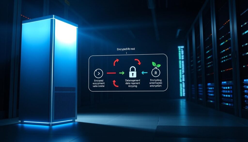
Redshift has several ways to protect your data. For data at rest, use cluster encryption with AWS Key Management Service (KMS). This encrypts your data blocks. For data in transit, use SSL connections to keep data safe.
Advanced users can encrypt data before loading it. Use column-level encryption for sensitive fields. Always update encryption keys every three months with KMS’s automatic rotation.
User Access Management
Begin with AWS Identity and Access Management (IAM) roles instead of root accounts. Here’s how to set up role-based access control (RBAC):
- Create IAM groups (e.g., “Analysts”, “Admins”)
- Attach specific Redshift permissions with JSON policies
- Assign users to groups instead of giving them direct access
Follow the least privilege principles. Only give access to what users need. For temporary access, use IAM’s temporary credentials.
Audit Logging Setup
Turn on Redshift’s audit logging through the AWS Console:
- Go to “Logging” in cluster configuration
- Choose an S3 bucket for log storage
- Set log retention policies (at least 90 days for compliance)
Connect with AWS CloudTrail for API call tracking. Use Redshift’s STL tables to watch user activity. Set up automated alerts for unusual login attempts.
Check access logs and encryption status with Amazon CloudWatch. Do security audits every quarter to keep policies up to date as your team grows.
Cost Management Strategies
Managing expenses is key when using cloud data warehouses. We’ll look at ways to keep costs down while keeping Redshift’s performance up for analytics.
Decoding the Pricing Structure
Amazon Redshift has two main pricing models: provisioned clusters and serverless options. The provisioned model charges for:
- Compute nodes (DC2/RA3 instances)
- Managed storage (RA3 only)
- Data transfer costs
Serverless pricing uses Redshift Processing Units (RPUs) with automatic scaling. Here’s a comparison of typical monthly costs:
| Pricing Model | Compute Cost | Storage Cost | Best For |
|---|---|---|---|
| Provisioned (dc2.large) | $0.25/hour | $0.024/GB | Predictable workloads |
| Serverless | $0.44/RPU-hour | $0.024/GB | Variable usage patterns |
Choosing between provisioned and serverless depends on workload consistency. For 1TB of data with daily queries, provisioned clusters can be 37% cheaper than serverless.
Smart Optimization Tactics
Here are some ways to cut costs:
- Right-size clusters: Use Amazon Compute Optimizer recommendations
- Enable auto-scaling: Match capacity to demand
- Compress data: Reduce storage needs by up to 60%
- Schedule queries: Leverage off-peak pricing
Use AWS Budgets to track costs. Set alerts when spending hits 75% of your budget to avoid surprises.
Reserved Instance Planning
Reserved Nodes (RNs) can save up to 75% over on-demand pricing. Here’s a break-even analysis:
| Commitment Term | Upfront Payment | Effective Hourly Rate | Break-Even Point |
|---|---|---|---|
| 1-year (No Upfront) | $0 | $0.18 | 7 months |
| 3-year (Partial Upfront) | $4,500 | $0.14 | 14 months |
Use Reserved Instances with Spot Instances for hybrid cost management. AWS’s Reserved Instance Recommendations tool can help find underutilized resources.
Integrating with BI Tools
To get the most out of your Redshift data warehouse, you need to connect it with business intelligence tools. These tools turn raw data into useful insights. They do this through easy-to-use dashboards and visualizations. Let’s look at three popular BI solutions that work well with Amazon Redshift.
Connecting Tableau to Redshift
Tableau is a great choice for Redshift users because of its strong analytics. Here’s how to connect securely:
- Install Tableau Desktop and open the “Connect” panel
- Select Amazon Redshift from the database options
- Enter your cluster endpoint, port (default: 5439), and credentials
Example connection string:
jdbc:redshift://your-cluster.region.redshift.amazonaws.com:5439/dev
Performance Tip: Use Tableau’s Extract Refresh feature for big datasets. It helps reduce the load on your cluster. Schedule extracts during quiet times using Tableau Server.
Using Amazon QuickSight With Redshift
QuickSight is perfect for beginners because it works well with AWS services. It has several benefits:
- Direct access through AWS Management Console
- Automatic schema discovery
- Pay-per-session pricing model
To improve performance, use SPICE for caching data. Also, limit visualizations to 5,000 rows unless you’re exporting the whole dataset.
Power BI Integration Steps
Microsoft’s Power BI connects to Redshift this way:
- Open Power BI Desktop > Get Data > Database
- Choose Amazon Redshift connector
- Input server address and authentication details
Pro Tip: Use DirectQuery mode for live analytics. But switch to Import mode for complex data changes. Watch query times in Power BI Service to find ways to improve.
| Tool | Connection Method | Best For | Cost Efficiency |
|---|---|---|---|
| Tableau | JDBC/ODBC | Enterprise reporting | $$$ |
| QuickSight | Native AWS | Quick deployments | $ |
| Power BI | Custom Connector | Microsoft ecosystems | $$ |
When picking a BI tool, think about your team’s skills and data needs. All three tools support scheduled refreshes. But QuickSight works best with AWS security. For those following this redshift tutorial step by step, start with QuickSight and then explore more advanced options.
Real-World Use Cases
Amazon Redshift helps businesses make better decisions by turning data into valuable assets. We’ll look at three ways beginners can use it to solve real problems. These examples show how the amazon redshift tutorial series leads to real results.
E-Commerce Analytics
Online stores use Redshift to understand their customers and sales. They collect data from:
- Web clickstreams
- Inventory systems
- Payment gateways
They use a query to find out who spends the most:
SELECT user_id, SUM(order_total) / COUNT(DISTINCT order_id)
FROM sales
GROUP BY 1
ORDER BY 2 DESC LIMIT 100;
This helps them target their marketing better. They see their queries run 25-40% faster than before.
IoT Data Processing
Redshift helps factories manage data from thousands of sensors. A typical setup includes:
- Streaming data via AWS IoT Core
- Processing in Kinesis Data Firehose
- Storing in Redshift every hour
An easy redshift tutorial for beginners shows how to average sensor readings:
SELECT device_id, AVG(sensor_value), COUNT(*)
FROM iot_readings
WHERE timestamp > NOW() - INTERVAL '1 hour'
GROUP BY 1;
This lets them keep an eye on their equipment and plan maintenance ahead.
Financial Reporting
Banks and fintech use Redshift for financial analysis. They set up their systems with:
- Encrypted S3 data lakes
- Row-level security
- Automated audit logs
They use window functions for monthly reports:
SELECT region,
SUM(revenue) OVER (PARTITION BY region ORDER BY month)
FROM financials
WHERE year = 2023;
This gives them insights into trends while keeping data safe. Redshift saves them 60% on storage costs.
Common Beginner Mistakes to Avoid
New Redshift users often make mistakes that affect performance and costs. We’ll look at three big errors and how to avoid them. We’ll use advice from experts to guide you.
Overprovisioning Clusters
Many beginners choose big clusters to be safe, but it’s expensive. A study found teams wasting $1,200 a month on 8-node DC2 clusters. They could have used 4-node RA3 instances instead. Here’s how to avoid this:
- Enable Concurrency Scaling for burst workloads
- Keep an eye on CloudWatch’s ClusterPercentageDiskSpaceUsed metric
- Start with smaller clusters and test them
| Scenario | Monthly Cost | Query Speed |
|---|---|---|
| 8-node Overprovisioned | $2,560 | 12 sec avg |
| 4-node Optimized | $1,280 | 14 sec avg |
Ignoring Compression
Not using compression means data takes up more space and queries are slower. AWS says:
Effective compression reduces storage needs while improving scan performance through smaller block sizes.
Always:
- Use COPY command’s automatic compression
- Check with ANALYZE COMPRESSION
- Choose AZ64 encoding for numeric columns
Poor Distribution Key Choices
Bad distribution keys can make one node handle most of the data. Here’s what to do:
- Use KEY distribution for large joined tables
- Apply ALL for small reference tables
- Use EVEN for tables in between
A financial client sped up queries by 65% by changing their transaction table to KEY distribution.
Conclusion
This amazon redshift tutorial for beginners teaches you the basics of cloud data warehouses. You’ve learned how to set up clusters, design schemas, and optimize queries. You also know how to use business intelligence tools.
These skills are essential for handling big data analytics in AWS. To get better, check out AWS training resources. Look into the Data Analytics Learning Path and certification programs.
Consider learning machine learning with Amazon SageMaker or spatial analytics with Redshift. Companies like Best Buy use Redshift for inventory forecasting. Fintech firms like Robinhood use it for transaction analysis.
Use the Redshift architecture diagram to understand how it works. Remember, success comes from proper distribution styles, vacuum operations, and compression encoding. Netflix and Airbnb use these strategies for their analytics environments.
Keep practicing with amazon redshift. Use AWS Cost Explorer to watch your costs. Join the AWS Developer Community to share tips with others. With time, you’ll move from basic SQL to designing big data solutions.
FAQ
How does Amazon Redshift’s columnar storage improve query performance?
Amazon Redshift stores data column-wise, which reduces I/O for analytical queries. This makes data compression up to 90% possible. For example, an e-commerce sales query only scans specific columns like category_id and sales_amount.
What’s the main difference between leader nodes and compute nodes?
The leader node parses SQL queries and develops plans. Compute nodes (in node slices) do parallel query processing. This MPP architecture handles large datasets efficiently. AWS documentation shows a single leader node can coordinate up to 128 compute nodes.
How do I choose between Redshift Serverless and provisioned clusters?
Serverless is good for variable workloads like monthly financial reports. Provisioned clusters are better for predictable high-volume workloads. AWS’s pricing calculator shows Serverless is cost-effective below 60% consistent cluster utilization.
What distribution style should I use for sales transaction tables?
Use KEY distribution for fact tables joined on common columns like order_id. Dimension tables use ALL distribution. Redshift Advisor recommends this for better join performance in retail analytics.
How does the COPY command handle S3 data loading errors?
The COPY command logs errors to a separate S3 bucket. Use JSON ‘auto’ for schema inference and MAXERROR 100 to prevent job failures. AWS Glue crawlers can validate data formats before loading.
When should I use materialized views versus regular views?
Materialized views improve performance for repetitive queries on stale data. Regular views are better for real-time data exploration. Financial reporting dashboards benefit from materialized views, achieving 5-8x faster response times.
How does Redshift Spectrum reduce query costs?
Spectrum queries S3 data directly without loading into Redshift. This reduces costs by only charging per TB scanned. It’s ideal for historical data queries.
What’s the most common mistake in WLM configuration?
Beginners often create too many queues (AWS recommends ≤8). This leads to underutilized resources. Use Concurrency Scaling for workload spikes. Monitor WLMQueueWaitTime in CloudWatch to adjust queues.
How do I secure sensitive data in Redshift?
Use AES-256 encryption with AWS KMS and SSL for data in transit. Implement RBAC through GRANT/REVOKE commands. For PCI compliance, create security views and audit access through CloudTrail.
What BI tool integrates best with Redshift for beginners?
Amazon QuickSight has native integration with Redshift. For Tableau/Power BI, use ODBC/JDBC drivers. Include TCPKeepAlive=true and SSL=require in connection strings for stable performance.
Why should I avoid using DISTSTYLE ALL for large tables?
DISTSTYLE ALL replicates full table data to every node, wasting storage. AWS documentation shows a 1TB table wastes 3TB in a 4-node cluster. Use it only for small dimension tables.
How often should I run VACUUM operations?
Run daily VACUUMs for tables with >5% deleted rows or heavy updates. Use v_acuum_sort_benefit to prioritize tables. For append-only tables, VACUUM is rarely needed – monitor via svv_table_info.


